

0 引言
近几十年来,国内外研究人员致力于解决非线性热传导问题。Annasabi等[6]使用B样条函数结合有限元法分析了非线性热传导问题。李腊梅等[12]将计算模型离散为块体和接触边界,提出一种非连续介质中热传导过程的数值模拟方法。刘承论等[13]利用边界元法计算了三维非稳态热传导问题。梁钰等[14]提出一种快速算法,并应用到导热系数随温度变化的瞬态热传导问题中。Sivin等[15]根据几何结构和问题的复杂程度,采用非标准网格技术对区域进行离散化,结合不动点迭代的比例边界有限元法求解了非线性瞬态热传导问题。Mierzwiczak等[16]基于Kirchhoff变换,将非线性热传导问题转化为线性,利用奇异边界元法成功求解了不规则区域中的稳态温度场。传统边界元法能够高效求解线性热传导问题。然而,对于非线性热传导问题,由于控制方程中通常包含与温度相关的非线性项,这些非线性项无法直接通过边界积分方程表示,导致传统边界元法难以直接应用。因此,必须采用特殊的方法来处理非线性问题,例如引入径向积分法、域分解技术或与其他数值方法耦合。Yang等[17]开发了新的径向积分边界元法(Radial Integration Boundary Element Method,RIBEM),并应用Newton-Raphson方法求解离散代数方程,计算了二维和三维非线性热传导问题。吴泽艳等[9]提出一种混合的无网格方法求解非线性瞬态热传导问题。Khosravifard等[18]采用了改进的无网格径向点插值方法,分析了涉及非均匀热源功能梯度材料的非线性瞬态传热问题。无网格法在计算非线性热传导中,其计算精度和效率与节点分布密切相关,节点布置不当容易出现计算效率低和不收敛的情况。
1991年,Shi[19]提出了NMM,包括数学覆盖和物理覆盖2套系统。通常以有限元的三角形或者四边形网格作为数学覆盖,共用一个节点的所有单元组成一个数学片,数学片被几何边界、材料界面或裂纹切割形成物理片,所有的物理片联结形成物理覆盖,物理覆盖需要精确的匹配问题域。物理片之间相互切割形成流形单元,流形单元是最小的积分单元。目前,NMM已经成功应用于热传导[20]、渗流[21]、裂纹扩展[22]、无界域问题[23]和边坡稳定性[24]等多个领域中。其中,在热传导计算中,胡国栋等[25]利用NMM研究了二维稳态功能梯度材料中的热传导问题。Zhang等[11]发展了无网格数值流形法求解功能梯度材料瞬态非线性热传导问题。Tan等[26]基于NMM模拟求解了稳态和瞬态热传导问题。Wang等[27]对NMM的局部网格进行加密,同时引入热力耦合模型研究岩石热破裂问题。Li等[28]创新性地将NMM应用于复杂工况下的压电材料分析,成功解决了机电荷载作用下含有任意形状孔洞缺陷的压电板的力学响应问题。Zhang[29]构建了三维土石混合体的数学模型,并将三维NMM应用于路基渗透性分析,为复杂地质条件下的路基渗透特性研究提供了新的方法。传统的有限元法在计算复杂边界问题时,网格容易产生畸变,导致计算精度下降并影响计算效率。NMM通过其独特的物理覆盖系统,能够精确描述复杂几何边界。此外,在材料界面处,NMM通过物理覆盖和局部函数,能够自然地描述不同材料间的热传导行为,无需引入额外的界面条件,从而简化了计算过程并提高了计算效率。本文首次构建了基于NMM的非线性稳态热传导离散格式,采用Newton-Raphson迭代算法对非线性方程组进行求解,并基于MATLAB软件实现数值求解过程。通过5个典型的算例验证了本文方法的正确性和鲁棒性,为非线性热传导问题的求解提供了一种新方法。
1 控制方程
如图1所示,二维问题域Ω由Dirichlet、Neumann和Robin三类边界条件所围成。
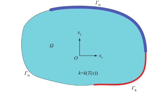
非线性稳态热传导的控制方程可以描述为二阶拟线性偏微分方程[20],即
式中:重复索引i在二维问题域中表示1, 2。T(x)表示问题域的温度;k(T)为随温度变化的导热系数;Q(x)是热源函数。
为了确定温度场,附加Dirichlet边界条件,即
Neumann边界条件为
Robin边界条件为
式中:ГD、 ГN、ГR分别为Dirichlet、Neumann和Robin边界;$\overline{T}$和$\stackrel{-}{q}$分别为ГD和ГN上给定的温度和热流量;h为换热系数;T∞是环境温度;n=(n1,n2)是单位外法向向量。
2 NMM求解非线性热传导
2.1 NMM简介
一般来讲,组成数学覆盖的数学片可以是任何形状,可以是有限元网格中共用1个节点的所有单元所组成,也可以是移动最小二乘法中节点的影响域。如图2所示,ABCD围成问题域Ω,EF为材料界面。以红色圆点所连接的四个有限单元构成1个数学片,用MPi表示,i=1,2,…,n;其中n表示数学片的个数。所有的数学片联结形成的数学覆盖须完全覆盖住问题域Ω。
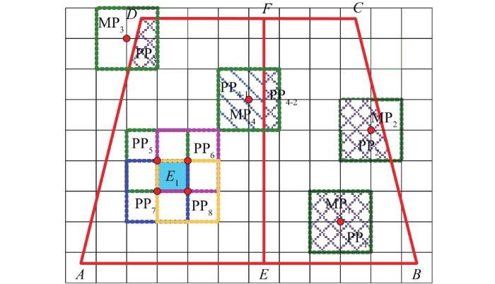
问题域边界和材料界面切割数学片形成物理片,1个数学片可以生成1个或者多个物理片。PPi-j是从数学片MPi中生成的第j个物理片,j=1,2,…,mi;其中,mi是指同一个数学片中生成物理片的个数。图2显示了3种典型的物理片:第1类物理片如PP1、PP5、PP6、PP7和PP8,它们由数学片MP1、MP5、MP6、MP7和MP8生成,这类物理片没有被切割,因此,第1类物理片就是数学片本身;第2类物理片如PP2、PP3,它是由数学片被边界切割并丢弃域外部分所形成;第3类物理片如PP4-1和PP4-2,是数学片MP4被材料界面EF切割生成的。一共生成np个物理片,所有的物理片组成了物理覆盖,精确覆盖问题域。物理片PP5、PP6、PP7和PP8的相互切割,最后形成了流形单元E1。当有限元网格用作数学覆盖时,流形单元是基本的积分单元。
对于每1个数学片,都有一个充分光滑的权函数wi(x)满足:
每一个物理片都有一个对应的权函数$\left\{{w}_{i-j}\right\}$,它取自数学片上的权函数在物理片上的限制,其表达式为
至此,构造出NMM的逼近u(x)为
式中:ui-j(x)代表物理片PPi-j的局部逼近,本文中ui-j(x)取未知常数。为简化表示,所有物理片都按单个指标排序,方程简化为
式中:N(x)是具有权函数的行向量,wi(x)为其中的元素;a=(ai),并且ai=u(xi)。
2.2 弱形式
Dirichlet边界条件是按照罚函数方法施加,带罚因子的弱形式为
温度T(x)采用分离变量法离散,
式中:T是所有物理片上未知温度的列向量。变分δT(x)可以近似为
通过将式(10)代入式(11),可以得到
式中:K(k(T))和F分别表示热传导矩阵和热荷载列阵,可以通过单元组装形成。在任意一个单元内Ke和Fe的形式分别为:
方程中的矩阵形式可以写为
其中,Bi=${\left(\begin{array}{ll}\frac{\partial {w}_{i}}{\partial {x}_{1}}& \frac{\partial {w}_{i}}{\partial {x}_{2}}\end{array}\right)}^{\mathrm{T}}$。
2.3 Newton-Raphson法
本文采用New-Raphson迭代方法,用来求解非线性方程组,残差可以定义为
R=F-KT 。
使用泰勒公式,可以得到
式中:Rn和Rn+1分别为第n和n+1次的残差。
取式(17)的线性项,可以得到下面的方程
式(16)对T的一阶偏导数为
式(19)右端第1项相对较小,可以忽略,只保留第2项,式(19)可以等价为
将式(20)代入式(18),并假定Rn+1为0,可以得出以下公式
然后,向量T可以更新为
式中θ被称为松弛因子,它的取值范围是0~1,旨在提高收敛性。在本文计算过程中,θ=1。
3 数值算例
本文提出了5个算例,用来验证NMM在非线性热传导问题中的计算精度。其中,第1个和第4个算例分别为规则四边形和矩形区域的热传导问题,均可以简化为有解析解的一维热传导模型。其余3个算例分别为矩形板中间含圆孔、二维不规则板、由2种材料组成的机械构件的热传导。为了评估数值结果,定义相对误差Re为
式中:T代表解析解或参考解;TNMM代表由NMM计算的数值解。
3.1 方板上的热传导
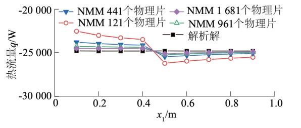
如图3所示的第1个算例,方板1.0 m×1.0 m上随温度变化的导热系数为k(T)=15+0.01T2,左、右2条边界上施加的温度分别为Tl=100 ℃, Tr=200 ℃。上、下2条边界为绝热边界。
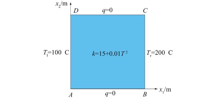
本算例采用的罚因子λ=1×10¹⁰。此算例可简化为一维热传导问题,推导出该算例的解析解[35]为
式中:a=24 833.3367; b=4 833.33。
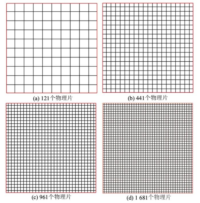
表1 物理片沿着x1方向的温度Table 1 Temperature distribution along x1 direction with different numbers of physical patches |
| x1/m | 不同数量物理片对应的温度/℃ | 解析解 温度/℃ | |||
|---|---|---|---|---|---|
| 121 | 441 | 961 | 1 681 | ||
| 0.1 | 118.325 5 | 118.388 7 | 118.412 4 | 118.424 8 | 118.451 6 |
| 0.2 | 132.746 6 | 132.776 4 | 132.787 3 | 132.792 9 | 132.806 3 |
| 0.3 | 144.733 1 | 144.746 9 | 144.751 8 | 144.754 4 | 144.761 0 |
| 0.4 | 155.102 1 | 155.107 2 | 155.109 0 | 155.109 9 | 155.112 6 |
| 0.5 | 164.305 3 | 164.305 3 | 164.305 3 | 164.305 3 | 164.305 3 |
| 0.6 | 172.607 6 | 172.611 5 | 172.612 8 | 172.613 4 | 172.615 1 |
| 0.7 | 180.214 1 | 180.220 4 | 180.222 4 | 180.223 4 | 180.225 9 |
| 0.8 | 187.253 1 | 187.260 9 | 187.263 4 | 187.264 6 | 187.267 4 |
| 0.9 | 193.819 0 | 193.827 7 | 193.830 6 | 193.831 9 | 193.834 8 |
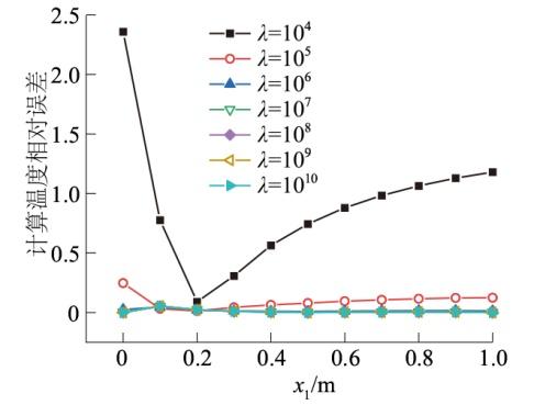
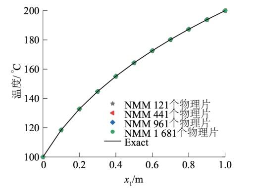
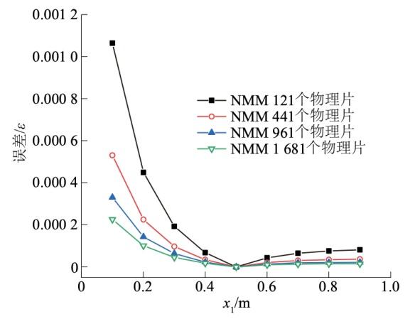
图7 解析解和不同物理片NMM计算的温度相对误差Fig.7 Relative errors of temperature between NMM results and analytic solution with different physical patches |
3.2 含圆孔矩形板的热传导
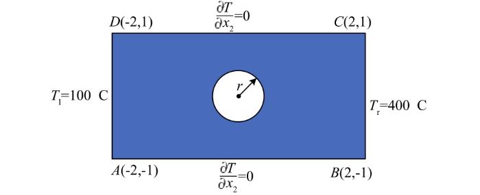
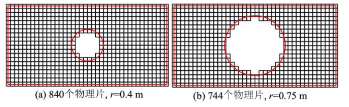
如图9所示,研究一个含有圆孔的矩形板,矩形板的尺寸为4.0 m×2.0 m,分析圆孔半径分别为r=0.4 m和r=0.75 m的2种情况。随温度变化的导热系数为k(T)=100+0.2T。左、右2条边界施加的温度分别为100 ℃和400 ℃,其他的边界都是绝热边界。本算例罚因子λ=1×10¹²。


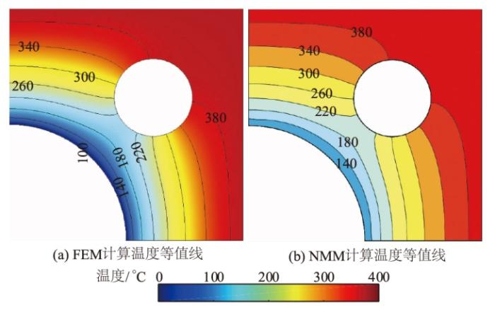
3.3 二维不规则板的热传导

如图14所示,采用NMM计算时,使用540个物理片覆盖问题域。考虑到几何模型和边界条件均具有对称特性,为提高计算效率,研究选取半圆形区域作为分析对象。计算过程中,迭代了8次,最后2次的误差为4.66×10⁻⁵。
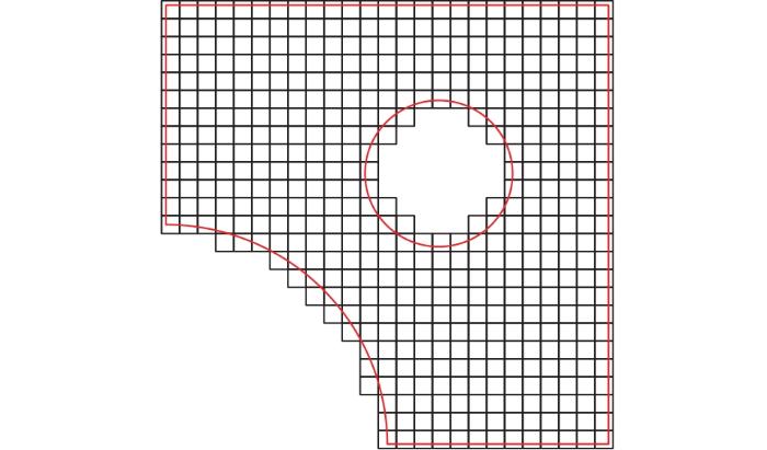

表2 半圆MN上的温度对比Table 2 Comparison of data along semicircle MN |
| 角度/(°) | 2种数值方法模拟的温度/℃ | 相对误差/% | |
|---|---|---|---|
| FEM | NMM | ||
| 0 | 206.212 | 206.189 | 0.010 8 |
| 15 | 213.797 | 214.249 | 0.211 4 |
| 30 | 234.151 | 233.911 | 0.102 6 |
| 45 | 261.848 | 261.402 | 0.170 1 |
| 60 | 291.467 | 290.781 | 0.235 5 |
| 75 | 319.142 | 318.279 | 0.270 5 |
| 90 | 342.639 | 342.345 | 0.085 8 |
| 105 | 361.005 | 360.606 | 0.110 5 |
| 120 | 374.235 | 373.799 | 0.116 7 |
| 135 | 382.982 | 382.663 | 0.083 4 |
| 150 | 388.234 | 387.971 | 0.067 8 |
| 165 | 390.946 | 390.748 | 0.050 7 |
| 180 | 391.773 | 391.636 | 0.035 1 |
3.4 含两层材料矩形板的热传导
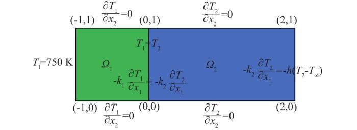
温度场可以简化为一维,只沿着x1方向发生变化,该问题的解析解[16]为:
式中:c=660.354 644 5 K; q=6 411.232 529 W/m2。
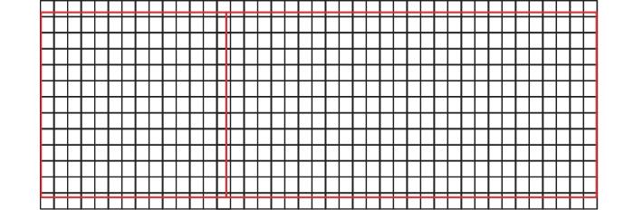
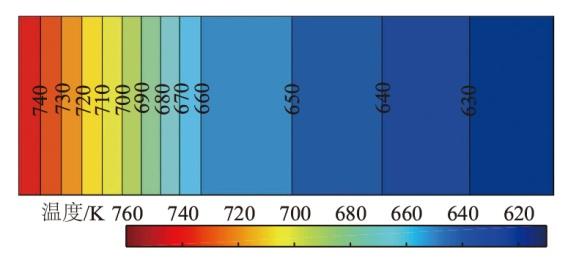
表3 沿着x1方向的温度Table 3 Temperatures along x1 direction |
| x1/m | 2种数值方法模拟的温度/K | 相对误差/10-5 | |
|---|---|---|---|
| NMM | 解析解 | ||
| -0.9 | 741.510 5 | 741.516 8 | 0.850 |
| -0.8 | 732.932 1 | 732.936 8 | 0.643 |
| -0.7 | 724.253 2 | 724.256 5 | 0.457 |
| -0.6 | 715.465 1 | 715.472 4 | 1.011 |
| -0.5 | 706.577 0 | 706.580 5 | 0.497 |
| -0.4 | 697.571 5 | 697.577 0 | 0.790 |
| -0.3 | 688.449 6 | 688.457 4 | 1.137 |
| -0.2 | 679.215 7 | 679.217 1 | 0.214 |
| -0.1 | 669.843 7 | 669.851 3 | 1.144 |
| 0 | 660.354 6 | 660.354 6 | 0.000 |
| 0.2 | 656.482 9 | 656.483 2 | 0.057 |
| 0.4 | 652.588 8 | 652.589 0 | 0.029 |
| 0.6 | 648.671 3 | 648.671 5 | 0.029 |
| 0.8 | 644.730 0 | 644.730 4 | 0.061 |
| 1.0 | 640.764 8 | 640.765 2 | 0.056 |
| 1.2 | 636.775 4 | 636.775 5 | 0.011 |
| 1.4 | 632.760 4 | 632.760 7 | 0.046 |
| 1.6 | 628.720 1 | 628.720 5 | 0.062 |
| 1.8 | 624.654 1 | 624.654 3 | 0.028 |
| 2 | 620.561 4 | 620.561 6 | 0.039 |

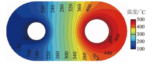
3.5 机械构件上的对流换热
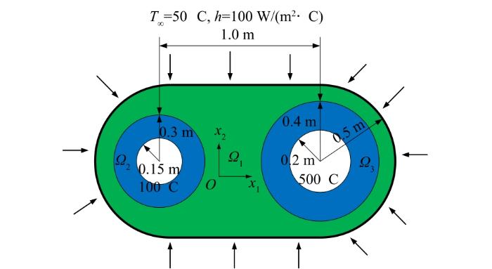
如图22所示,此构件采用四边形网格作为数学覆盖,经过材料边界和几何边界切割后,生成792个物理片。由于此算例几何形状较为复杂,解析解不易求得,因此将采用有限元软件ANSYS计算相应结果作为对比,ANSYS软件采用八节点二次单元对问题域进行离散。有限元模型所用单元数总计476个,节点总数为1 149个。
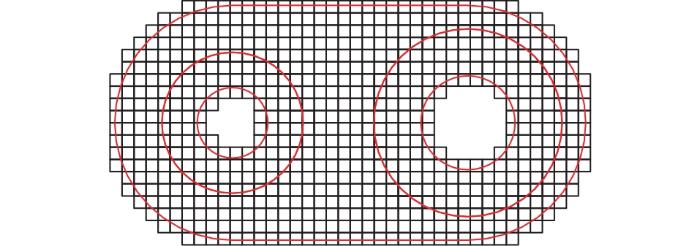
表4 界面圆环上的温度计算结果及对比Table 4 Calculated temperature results and comparison along interface ring |
| 角度/ (°) | 左边的界面圆环 | 右边的界面圆环 | ||||
|---|---|---|---|---|---|---|
| 温度/℃ | 相对误 差/% | 温度/℃ | 相对误 差/% | |||
| ANSYS | NMM | ANSYS | NMM | |||
| 0 | 256.32 | 255.19 | 0.442 | 451.69 | 451.87 | 0.040 |
| 22.5 | 248.49 | 247.77 | 0.288 | 450.65 | 450.74 | 0.019 |
| 45.0 | 227.69 | 227.25 | 0.192 | 447.11 | 447.32 | 0.046 |
| 67.5 | 200.23 | 199.99 | 0.117 | 439.59 | 439.72 | 0.030 |
| 90.0 | 173.61 | 173.29 | 0.186 | 424.92 | 424.93 | 0.002 |
| 112.5 | 153.16 | 152.86 | 0.193 | 400.40 | 400.65 | 0.062 |
| 135.0 | 139.73 | 139.491 | 0.175 | 373.54 | 373.84 | 0.080 |
| 157.5 | 132.23 | 131.93 | 0.230 | 354.18 | 354.02 | 0.046 |
| 180.0 | 129.83 | 129.27 | 0.432 | 347.26 | 347.50 | 0.069 |
4 结束语
本文采用四边形网格覆盖的NMM求解二维非线性稳态热传导问题,通过连续材料、含圆孔的非连续材料以及非均值材料等典型算例,系统验证了NMM方法的可行性和计算精度。与传统FEM相比,NMM在模拟不规则问题域热传导方面具有显著优势。这种优势主要源于NMM独特的数值特性:在NMM中,插值子域与积分子域相互独立,而FEM中2种子域是相同的。此外,NMM能够精确地描述复杂几何边界,并充分利用局部域中解的行为特征,这使得其在裂纹扩展模拟方面展现出比FEM更强的灵活性。基于当前研究成果,后续研究致力于将NMM方法拓展至二维热裂纹问题中。